 Once one comes to the sobering conclusion that they are in fact slaves to money and they need to declare “DEBT TOTAL WAR”, the question then becomes: “Where do I/we go from here?”.
The first step in unleashing debt total war is to understand where your money is going. This is best accomplished by creating a Monthly Summary. This is the first weapon in the arsenal of financial freedom.
We began a monthly summary in 2007 shortly after moving back from Japan. We were amazed at how poorly we understood where our money was going until we started capturing it and looking at it through the lense of a holy warrior. Suddenly our enemy’s finger prints could be seen…and of course, the enemy was us! When we looked at the numbers we were actually adding about $65.00/mth onto the credit card debt. Knowledge is power…and applying that knowledge to our monthly finances became very powerful indeed. During the course of debt total war we went from going $65 further into the hole to paying off $1000 of debt each month.
Step 1. Get a Spreadsheet Program
![]() The funny thing is, that while we were swimming in debt I thought we’d be savvy and buy Quicken so we could track our expenditures because we could hook it direct into our bank account. Did you catch what I said in the previous sentence? I said “we’d be savvy and BUY Quicken”…just so you know…the answer to reducing costs is not by increasing them. What I found out was that Quicken was not going to be flexible enough for the granularity we wanted. So we ended up ditching Quicken and using good old Microsoft Excel which we already owned on our home computer. Of course there are lots more options available now such as Google Docs, Star Office but suffice it to say that some sort of spreadsheet software will be required.
The funny thing is, that while we were swimming in debt I thought we’d be savvy and buy Quicken so we could track our expenditures because we could hook it direct into our bank account. Did you catch what I said in the previous sentence? I said “we’d be savvy and BUY Quicken”…just so you know…the answer to reducing costs is not by increasing them. What I found out was that Quicken was not going to be flexible enough for the granularity we wanted. So we ended up ditching Quicken and using good old Microsoft Excel which we already owned on our home computer. Of course there are lots more options available now such as Google Docs, Star Office but suffice it to say that some sort of spreadsheet software will be required.
Next you want to set up your spreadsheet with four tabs:
- Roll Up (Tab1) – Used for calculating the data from Month 1 (Tab2)
- Month 1 (Tab2) – Used for capturing account transactions and categorizing (using lists from Income and Expenses) them
- Income (Tab3) – Used for Income Categories
- Expense (Tab4) – Used for Expense Categories

1.1 Spreadsheet Tabs
Step 2. Get the Data
Once you’ve sourced a spreadsheet program and setup the tabs you will need to get the data. Almost all Canadian banks allow you to download your account activity in what is called “comma separated value” format or .csv file that contains all of your debits and credits. After you have downloaded the data you can copy and paste it into the Month 1 tab. NOTE: It’s best to wait a few days after the end of the month before downloading the data as there can be a few adjustments especially if the end of the month is on a weekend.

2.1 Tab 1 – The Raw Data pasted into the Month 1 tab.
You should have something like this (I’ve removed the account number and changed the actual amounts to a generic fives):
Step 3. Set up Categories
Ok so now you have a spreadsheet with your income and expense data. Next you need to categorize the data so you can roll up the amounts and eventually create your budget. We have continually updated our categories over time (which is why using a flexible tool like a spreadsheet is so helpful and also why Quicken didn’t work so well for us) so for our example here I am going to use generic categories from finiki (http://www.finiki.org/wiki/Budgeting) but you can customize to fit your needs. You will need two sets of categories; income and expenses.
Sample Income Categories (Tab 2)
Salary
Canada Child Tax Benefit (CCTB)
Other
Sample Expense Categories (Tab 3)
Home
Rent or mortgage payments
Property taxes/condo fees
Home insurance
Utilities (such as electricity, water, cable or telephone)
Repairs and maintenance
Transportation
Public transportation
Car loan payments
Car repairs, gas, etc.
Car insurance/registration, etc
Living expenses
Groceries
Child care
Medical and dental
Outstanding loan payments
Basic clothing
Life, disability and medical insurance
Emergency fund
Other
Step 4. Define Names
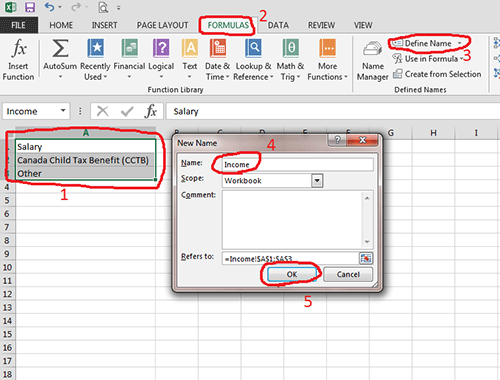
You should now have 3 tabs in your spreadsheet and now you need to make the categories from tabs 2 and 3 available for use on tab 1. In Excel this can be done via a drop down list (http://office.microsoft.com/en-ca/excel-help/create-or-remove-a-drop-down-list-HP005202215.aspx). Go to tab 2 and highlight the three entries and then go to the FORMULAS section of the ribbon and in the Defined Names section click on “Define Name”.

4.1 – Tab 2 – Setting Define Name for Income Categories

4.2 – Tab 3 – Setting Define Name for Expenses categories
Step 5. Categorize the Data
Now that you have the categories available we need to categorize the data we downloaded from the bank in step 2 and added into the Month 1 tab.

5.1 Click on the cell you want to set a drop down for. Click on the Data Tab then on “Data Validation” and then on “Data Validation”.

5.2 Once in the Data Validation window under validation criteria click on the “Allow” drop down and click on “List”. Then in the “Source” field type in “=Expenses” (using the name we set up in Step 3) and then click OK.

5.3 Now you should have a drop down list available using the Defined Name.

5.4 Repeat steps 5.1 and 5.2 for all other cells in the Expenses column. Do the same for the income column except when you go to enter in the “Source” field set it to “=Income”. Then assign each amount a category.

5.5 I’ve added some formatting (https://support.office.com/client/format-numbers-0afe8f52-97db-41f1-b972-4b46e9f1e8d2). For example I have formatted the Amount entries as currency to make the debits red and credits black to make it a little more human friendly.
Step 6. Roll Up the Data
We’ve got the ability to capture and categorize our data but we still need to be able to roll it up so we can get the full picture. We do this by building a roll up sheet that can scan the Month 1 tab and sum its contents based on its category.

6.1 Add in Category rows on the Roll Up tab and create columns for each month (I am only showing data for Month 1 but you would build the sheets for all 12 months).

6.2 Next we need to sum the categories from the Month1 tab into the corresponding cells in the Roll Up tab. This is accomplished with the “Sumif” function in Excel (https://support.office.com/en-NZ/article/SUMIF-5fd078db-e5f8-4726-b08f-74fd0064e7fe). We are going to tell Excel that we want to scan the Month 1 tab and if the Income column (F) is set to “Salary” then we want to sum the Amount column (D) entries and put them in the “Salary” row (3) entry for Month 1. The formula will look like this: =SUMIF(‘Month 1’!F2:F250,”=Salary”, ‘Month 1’!D2:D250). This formula will scan from row 2 up to row 250 on the Month 1 tab but you can modify as needed based on how you setup your own sheets.
Income Queries
Canadian Child Tax Benefit
=SUMIF(‘Month 1’!F2:F250,”=Canada Child Tax Benefit (CCTB)”, ‘Month 1’!D2:D250)
Other
=SUMIF(‘Month 1’!F2:F250,”=Other”, ‘Month 1’!D2:D250)
Expense Queries
The expenses column is E on the Month 1 tab so we need to modify our queries accordingly. Enter these queries into their corresponding cell numbers.
Rent or mortgage payments (Cell B9)
=SUMIF(‘Month 1’!E2:E250,”=Rent or mortgage payments”, ‘Month 1’!D2:D250)
Property taxes/condo fees (Cell B10)
=SUMIF(‘Month 1’!E2:E250,”=Property taxes/condo fees”, ‘Month 1’!D2:D250)
Home insurance (Cell B11)
=SUMIF(‘Month 1’!E2:E250,”=Home insurance”, ‘Month 1’!D2:D250)
Utilities (such as electricity, water, cable or telephone) (Cell B12)
=SUMIF(‘Month 1’!E2:E250,”=Utilities (such as electricity, water, cable or telephone)”, ‘Month 1’!D2:D250)
Repairs and maintenance (Cell B13)
=SUMIF(‘Month 1’!E2:E250,”=Repairs and maintenance”, ‘Month 1’!D2:D250)

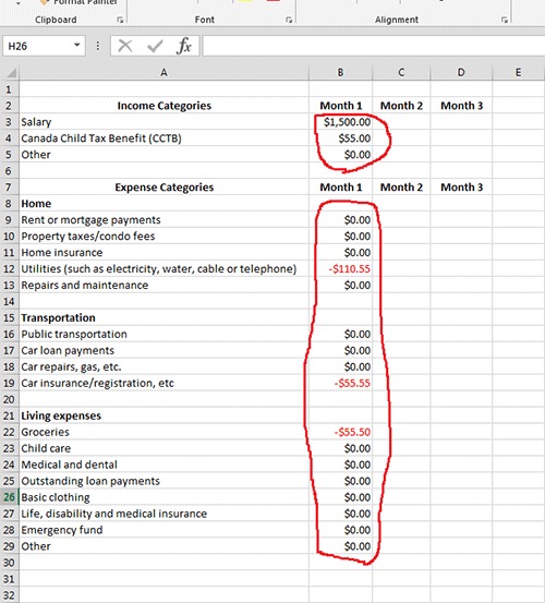
6.3 Roll Up tab with all categories being rolled up from the Month 1 tab. I also formatted them similar to step 5.5.

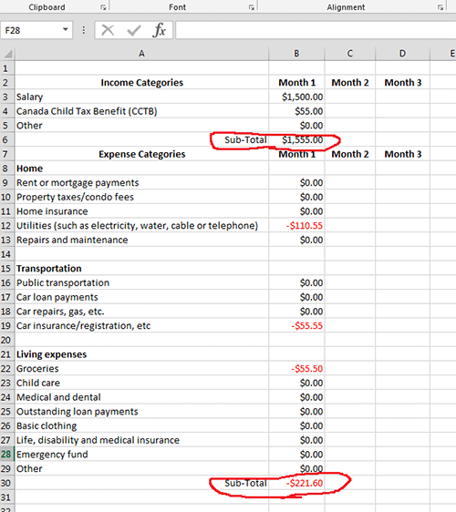
6.4 Next we need to add in sub-totals to sum the Income and Expense. For income in cell B6 type in “=SUM(B3:B5)” without the quotes of course. In cell B30 type in “=SUM(B9:B29)”.

6.5 Finally, we add in a Plus or Minus cell to show whether we are spending more than we make. In cell B32 type in “=B6+B30”.
7. Monthly Summary Complete
Are you still with us? If yes, you’ve just completed the building blocks for a monthly summary. You can use these building blocks to build out a custom spreadsheet to your own personal preferences including one tab for each month. Once your spreadsheet is setup and you are downloading data from your bank you can then move onto Phase 2 which is to setup budgets for the categories you created in Phase 1.
REMEMBER: the categories are not set in stone…you can update them anytime depending on your preferences but be sure to update anything that is linked in your spreadsheet (or do what we do and implement changes at the beginning of the new year so you don’t have to go back and remediate the current year’s data).
Attached below is the example monthly summary we built above (Excel 2013 format):
